The lineup() plan - align an axis with a signal

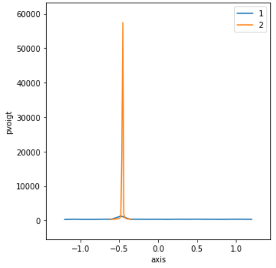
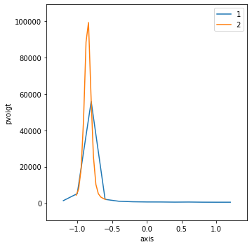
In this example, we demonstrate the apstools.plans.lineup() plan, which aligns an axis using some statistical measure (cen: centroid, com: center of mass, max: position of peak value, or even min: negative trending peaks) of a signal. If an alignment is possible, an optional rescan will fine-tune the alignment within the width and center of the first scan. Use rescan=False keyword to disable. Here’s an example chart showing the first (roughly, locate at least one point within the peak) and second (fine-tune the position) scans.

We’ll use a floating-point scalar value (not connected to hardware) as a positioner. Then, we prepare a simulated detector signal that is a computation based on the value of our positioner. The computed signal is a model of a realistic diffraction peak (pseudo-Voigt, a mixture of a Gaussian and a Lorentzian) one might encounter in a powder diffraction scan. The model peak is a pseudo-voigt function to which some noise has been added. Random numbers are used to modify the ideal pseudo-voigt function so as to simulate a realistic signal.

For this demo, we’ll use a temporary databroker catalog (deleted when the notebook is closed) since we do not plan to review any of this data after collection. We’ll display the data during the scan(in both a table and a chart) using a BestEffortCallback() subscription to the bluesky.RunEngine().

from apstools.devices import SynPseudoVoigt
from apstools.plans import lineup
from bluesky import RunEngine
from bluesky.callbacks import best_effort
import bluesky.plan_stubs as bps
import databroker
import numpy
import ophyd

bec = best_effort.BestEffortCallback()
cat = databroker.temp()
RE = RunEngine({})
RE.subscribe(cat.v1.insert)
RE.subscribe(bec)

1

Setup

Set the IOC prefix and connect with our EPICS PVs.

IOC = "gp:"
axis = ophyd.EpicsSignal(f"{IOC}gp:float1", name="axis")

axis.wait_for_connection()

Once connected, create the detector signal (the computed pseudo-Voigt) with default peak parameters.

# Need to know that axis is connected before using here.
pvoigt = SynPseudoVoigt(name="pvoigt", motor=axis, motor_field=axis.name)

The pvoigt signal must have kind="hinted" for it to appear in tables and plots.

pvoigt.kind = "hinted"

Move axis to a starting position. Pick zero.

RE(bps.mv(axis, 0))

()

Scan

To make things interesting, first randomize the peak parameters. (Peak is placed randomly between -1..+1 on axis scale, with random width, scale, pseudo-Voigt mixing parameter, noise, …)

pvoigt.randomize_parameters(scale=100_000)

Run the lineup() plan through the range where the peak is expected. Don’t need many points to catch some value that is acceptable (max is more than 4*min) the background.

RE(lineup(pvoigt, axis, -1.2, 1.2, 13, feature="cen", rescan=True))
print(f"{pvoigt.read()=}, {axis.get()=}")

Transient Scan ID: 1     Time: 2022-09-28 15:35:18
Persistent Unique Scan ID: '22182d47-72c1-450b-bf62-035a2c608d11'
New stream: 'primary'
+-----------+------------+------------+------------+
|   seq_num |       time |       axis |     pvoigt |
+-----------+------------+------------+------------+
|         1 | 15:35:18.6 |    -1.2000 |       1413 |
|         2 | 15:35:18.6 |    -1.0000 |       5259 |
|         3 | 15:35:18.7 |    -0.8000 |      55856 |
|         4 | 15:35:18.7 |    -0.6000 |       2113 |
|         5 | 15:35:18.7 |    -0.4000 |       1070 |
|         6 | 15:35:18.8 |    -0.2000 |        796 |
|         7 | 15:35:18.8 |     0.0000 |        689 |
|         8 | 15:35:18.8 |     0.2000 |        675 |
|         9 | 15:35:18.8 |     0.4000 |        600 |
|        10 | 15:35:18.8 |     0.6000 |        649 |
|        11 | 15:35:18.9 |     0.8000 |        567 |
|        12 | 15:35:18.9 |     1.0000 |        547 |
|        13 | 15:35:18.9 |     1.2000 |        552 |
+-----------+------------+------------+------------+
generator rel_scan ['22182d47'] (scan num: 1)





Transient Scan ID: 2     Time: 2022-09-28 15:35:19
Persistent Unique Scan ID: '9928a319-fa14-4b5e-837f-1f4058f7029c'
New stream: 'primary'
+-----------+------------+------------+------------+
|   seq_num |       time |       axis |     pvoigt |
+-----------+------------+------------+------------+
|         1 | 15:35:19.1 |    -1.0154 |       4403 |
|         2 | 15:35:19.1 |    -0.9801 |       7746 |
|         3 | 15:35:19.1 |    -0.9447 |      18831 |
|         4 | 15:35:19.2 |    -0.9093 |      46123 |
|         5 | 15:35:19.2 |    -0.8739 |      88448 |
|         6 | 15:35:19.2 |    -0.8386 |      99186 |
|         7 | 15:35:19.2 |    -0.8032 |      59675 |
|         8 | 15:35:19.2 |    -0.7678 |      25649 |
|         9 | 15:35:19.3 |    -0.7325 |      10329 |
|        10 | 15:35:19.3 |    -0.6971 |       5200 |
|        11 | 15:35:19.3 |    -0.6617 |       3386 |
|        12 | 15:35:19.3 |    -0.6263 |       2602 |
|        13 | 15:35:19.3 |    -0.5910 |       2046 |
+-----------+------------+------------+------------+
generator rel_scan ['9928a319'] (scan num: 2)



pvoigt.read()={'pvoigt': {'value': 2046, 'timestamp': 1664397319.3793561}}, axis.get()=-0.8496701712914874

Validate

Show the position after the lineup() completes. Test (Python assert) that it is within the expected range.

center = pvoigt.center
sigma = 2.355 * pvoigt.sigma
print(f"{center=}\n{sigma=}\n{bec.peaks=}")
assert center-sigma <= axis.get() <= center+sigma

center=-0.8503901139652472
sigma=0.11456520969899238
bec.peaks={
'com':
    {'pvoigt': -0.8461974129441658}
,
'cen':
    {'pvoigt': -0.8496701712914874}
,
'max':
    {'pvoigt': (-0.8385705807871623,
                99186)}
,
'min':
    {'pvoigt': (-0.5909727956676526,
                2046)}
,
'fwhm':
    {'pvoigt': 0.11177564414922392}
,
}