Plot x, y data from a databroker run

This Bluesky notebook only uses the databroker package (and matplotlib) to plot \((x,y)\) data from a previous measurement.

1. Show what data catalogs are available

import databroker
list(databroker.catalog)

['bdp2022',
 'class_2021_03',
 '6idb_export',
 'apstools_test',
 'class_data_examples',
 'usaxs_test',
 'korts202106',
 'training']

2. Choose a specific run from a catalog

Here, the class_data_examples catalog will be used.

We create an instance of this catalog and assign it to the variable cat. In this cat, the run with scan_id=86 has a scan of detector vs. motor. The cat object is like a dictionary where scan_id can be used as a key. Next, using 86 as the key, we create an object called run that will be used to access the data from this run.

cat = databroker.catalog["class_data_examples"]
run = cat[86]
run

BlueskyRun
  uid='d19530f7-1ca6-4c02-a83b-229b3d92b6d1'
  exit_status='success'
  2021-03-06 14:10:46.462 -- 2021-03-06 14:10:49.317
  Streams:
    * baseline
    * primary

3. Show the (primary) data

Get all the data available from the primary stream. The primary stream is where bluesky stores the data acquired from a scan. databroker returns this data as an xarray Dataset.

The detector is named noisy and the motor is named m1. We’ll refer to m1 and noisy as data variables to be consistent with the xarray.Dataset (as shown in the table below).

dataset = run.primary.read()
dataset

<xarray.Dataset>
Dimensions:           (time: 23)
Coordinates:
  * time              (time) float64 1.615e+09 1.615e+09 ... 1.615e+09 1.615e+09
Data variables:
    m1                (time) float64 0.939 0.941 0.942 ... 0.968 0.969 0.971
    m1_user_setpoint  (time) float64 0.9392 0.9407 0.9421 ... 0.9693 0.9708
    noisy             (time) float64 8.589e+03 1.067e+04 ... 1.076e+04 8.774e+03

xarray.Dataset

• Dimensions:
  • time: 23
• Coordinates: (1)
  • time
    (time)
    float64
    1.615e+09 1.615e+09 ... 1.615e+09

    array([1.615061e+09, 1.615061e+09, 1.615061e+09, 1.615061e+09, 1.615061e+09,
           1.615061e+09, 1.615061e+09, 1.615061e+09, 1.615061e+09, 1.615061e+09,
           1.615061e+09, 1.615061e+09, 1.615061e+09, 1.615061e+09, 1.615061e+09,
           1.615061e+09, 1.615061e+09, 1.615061e+09, 1.615061e+09, 1.615061e+09,
           1.615061e+09, 1.615061e+09, 1.615061e+09])

• Data variables: (3)
  • m1
    (time)
    float64
    0.939 0.941 0.942 ... 0.969 0.971

    object :

    m1

    array([0.939, 0.941, 0.942, 0.944, 0.945, 0.946, 0.948, 0.949, 0.951,
           0.952, 0.954, 0.955, 0.956, 0.958, 0.959, 0.961, 0.962, 0.964,
           0.965, 0.966, 0.968, 0.969, 0.971])

  • m1_user_setpoint
    (time)
    float64
    0.9392 0.9407 ... 0.9693 0.9708

    object :

    m1

    array([0.93922358, 0.9406578 , 0.94209202, 0.94352624, 0.94496046,
           0.94639468, 0.9478289 , 0.94926312, 0.95069734, 0.95213156,
           0.95356578, 0.955     , 0.95643422, 0.95786844, 0.95930266,
           0.96073688, 0.9621711 , 0.96360532, 0.96503954, 0.96647376,
           0.96790798, 0.9693422 , 0.97077642])

  • noisy
    (time)
    float64
    8.589e+03 1.067e+04 ... 8.774e+03

    object :

    noisy

    array([ 8589.32940855, 10673.5935127 , 12175.42592515, 16002.50003937,
           19570.16387909, 22262.12759241, 32683.26999595, 37632.86194784,
           56726.20388132, 70195.36934214, 91437.94502751, 97870.56104504,
           92105.54803581, 69931.50593825, 57654.64241544, 40947.06521792,
           31686.60297804, 22357.10017001, 19497.85944574, 17007.29364564,
           12802.50606181, 10761.63637859,  8773.96384533])

• Attributes: (0)

4. Get data for the \(x\) and \(y\) axes

The plotting steps become easier (and more general) if we create objects for each specific data variable to be plotted.

Pick the m1 (motor readback value) and noisy data for \(x\) and \(y\), respectively.

x = dataset["m1"]
y = dataset["noisy"]

5. Use MatPlotLib

import matplotlib.pyplot as plt

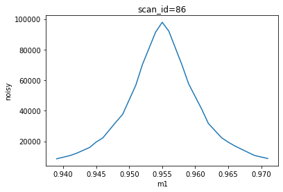
6. Plot \((x,y)\) using matplotlib

Follow the MatPlotLib tutorial to learn how to customize this plot. The data (x.values and y.values) are obtained as numpy ndarrays.

plt.plot(x.values, y.values)
plt.xlabel(x.name)
plt.ylabel(y.name)
plt.title(f"scan_id={run.metadata['start']['scan_id']}")

Text(0.5, 1.0, 'scan_id=86')

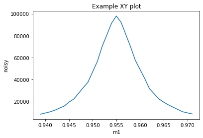
7. Plotting function

Summarizing the code above, here is a handy function you can use to plot such \((x, y)\) data. Or, you can use this code as a starting point to make your own plot function.

def xyplot(dataset, xname, yname, title=None):
    """
    Plot the data from the primary stream (above).

    Example::

        xyplot(cat[-1].primary.read(), x.name, y.name)
    """
    import matplotlib.pyplot as plt

    x = dataset[xname]
    y = dataset[yname]
    title = title or f"{yname} v. {xname}"

    plt.plot(x.values, y.values)
    plt.title(title)
    plt.xlabel(xname)
    plt.ylabel(yname)

Here is an example using this function with the dataset from above. The actual name for each data variable must match the name provided by the dataset. A plot title is provided.

xyplot(dataset, "m1", "noisy", title="Example XY plot")