XAFS scan

From APS Python Training for Bluesky Data Acquisition.

Objective

Example multi-segment XAFS scan. A full scan might be divided into:

region	steps	units	count time
pre-edge	constant energy	keV	constant
near-edge	constant energy	eV	constant
low k	constant k	1/angstrom	constant
higher k	constant k	1/angstrom	scales with k

For the higher k region, the count time is computed as:

preset_time = requested_time * (1 + factor*k**exponent)

where exponent=0.5, factor=2.0, and requested_time is the time specified by the caller.

note: We are connected to simulated hardware. The simulated scalers generate random pulses. All detector data is random numbers.

Start the instrument package

Our instrument package is in the bluesky subdirectory here so we add that to the search path before importing it.

import pathlib, sys
sys.path.append(str(pathlib.Path.home() / "bluesky"))
from instrument.collection import *

RE.waiting_hook = None  # disable the progress bar, looks awful in notebooks

/home/prjemian/bluesky/instrument/_iconfig.py
Activating auto-logging. Current session state plus future input saved.
Filename       : /home/prjemian/Documents/projects/BCDA-APS/bluesky_training/docs/source/howto/.logs/ipython_console.log
Mode           : rotate
Output logging : True
Raw input log  : False
Timestamping   : True
State          : active

I Thu-18:16:30 - ############################################################ startup
I Thu-18:16:30 - logging started
I Thu-18:16:30 - logging level = 10
I Thu-18:16:30 - /home/prjemian/bluesky/instrument/session_logs.py
I Thu-18:16:30 - /home/prjemian/bluesky/instrument/collection.py
I Thu-18:16:30 - CONDA_PREFIX = /home/prjemian/.conda/envs/bluesky_2023_2

Exception reporting mode: Minimal

I Thu-18:16:30 - xmode exception level: 'Minimal'
I Thu-18:16:30 - /home/prjemian/bluesky/instrument/mpl/notebook.py
I Thu-18:16:30 - #### Bluesky Framework ####
I Thu-18:16:30 - /home/prjemian/bluesky/instrument/framework/check_python.py
I Thu-18:16:30 - /home/prjemian/bluesky/instrument/framework/check_bluesky.py
I Thu-18:16:30 - /home/prjemian/bluesky/instrument/framework/initialize.py
I Thu-18:16:30 - RunEngine metadata saved in directory: /home/prjemian/Bluesky_RunEngine_md
I Thu-18:16:30 - using databroker catalog 'training'
I Thu-18:16:30 - using ophyd control layer: pyepics
I Thu-18:16:30 - /home/prjemian/bluesky/instrument/framework/metadata.py
I Thu-18:16:30 - /home/prjemian/bluesky/instrument/epics_signal_config.py
I Thu-18:16:30 - Using RunEngine metadata for scan_id
I Thu-18:16:30 - #### Devices ####
I Thu-18:16:30 - /home/prjemian/bluesky/instrument/devices/area_detector.py
I Thu-18:16:30 - /home/prjemian/bluesky/instrument/devices/calculation_records.py
I Thu-18:16:33 - /home/prjemian/bluesky/instrument/devices/fourc_diffractometer.py
I Thu-18:16:33 - /home/prjemian/bluesky/instrument/devices/ioc_stats.py
I Thu-18:16:33 - /home/prjemian/bluesky/instrument/devices/kohzu_monochromator.py
I Thu-18:16:33 - /home/prjemian/bluesky/instrument/devices/motors.py
I Thu-18:16:33 - /home/prjemian/bluesky/instrument/devices/noisy_detector.py
I Thu-18:16:34 - /home/prjemian/bluesky/instrument/devices/scaler.py
I Thu-18:16:34 - /home/prjemian/bluesky/instrument/devices/shutter_simulator.py
I Thu-18:16:34 - /home/prjemian/bluesky/instrument/devices/simulated_fourc.py
I Thu-18:16:34 - /home/prjemian/bluesky/instrument/devices/simulated_kappa.py
I Thu-18:16:34 - /home/prjemian/bluesky/instrument/devices/slits.py
I Thu-18:16:34 - /home/prjemian/bluesky/instrument/devices/sixc_diffractometer.py
I Thu-18:16:35 - /home/prjemian/bluesky/instrument/devices/temperature_signal.py
I Thu-18:16:35 - #### Callbacks ####
I Thu-18:16:35 - /home/prjemian/bluesky/instrument/callbacks/spec_data_file_writer.py
I Thu-18:16:35 - #### Plans ####
I Thu-18:16:35 - /home/prjemian/bluesky/instrument/plans/lup_plan.py
I Thu-18:16:35 - /home/prjemian/bluesky/instrument/plans/peak_finder_example.py
I Thu-18:16:35 - /home/prjemian/bluesky/instrument/utils/image_analysis.py
I Thu-18:16:35 - #### Utilities ####
I Thu-18:16:35 - writing to SPEC file: /home/prjemian/Documents/projects/BCDA-APS/bluesky_training/docs/source/howto/20230413-181635.dat
I Thu-18:16:35 -    >>>>   Using default SPEC file name   <<<<
I Thu-18:16:35 -    file will be created when bluesky ends its next scan
I Thu-18:16:35 -    to change SPEC file, use command:   newSpecFile('title')
I Thu-18:16:35 - #### Startup is complete. ####

We’ll use these later. Import now.

from ophyd import EpicsSignalRO

import math
import numpy as np
import pandas as pd

Energy & k

The Kohzu monochromator support expects energy in keV and wavelength in 1/angstrom. XAFS is similar, k in 1/angstrom, but also uses eV sometimes for energy. We need to be flexible.

Fundamental physical constants are provided by the scipy package. The Python pint package is used to provide unit conversions that will help to convert between energy and k coordinates. With these two packages, our software provides flexibility for the units a caller must use. And the code we use documents itself about our choice of units.

Here we define routines to convert between energy and k.

import pint
import scipy.constants

ureg = pint.UnitRegistry()
Qty = ureg.Quantity  # a shortcut

hbar = Qty(scipy.constants.hbar, "J Hz^-1")
electron_mass = Qty(scipy.constants.m_e, "kg")
TWO_M_OVER_HBAR_SQR = 2 * electron_mass / (hbar**2)


def energy_to_k(E, E0):
    energy_difference = Qty(E - E0, "keV")
    kSqr = (TWO_M_OVER_HBAR_SQR * energy_difference).to("1/angstrom^2")
    return math.sqrt(kSqr.magnitude)


def k_to_energy(k, E0):
    """
    k = sqrt( (2m(E-E0)) / hbar^2) = sqrt( const * (E-E0))
    """
    k_with_units = Qty(k, "1/angstrom")
    edge_keV = Qty(E0, "keV")
    energy_difference = (k_with_units**2 / TWO_M_OVER_HBAR_SQR).to("keV")
    return (energy_difference + edge_keV).magnitude

Multiple segments

XAFS scans measure signals from two or more detectors as the incident X-ray energy is varied. One method is to step the energy where the step size is different depending on the region of the scan. Steps could be in constant units of energy or k (see above).

We define here a default list of four regions (known here as segments), each showing a different feature of units or count time weighting. This default list is used in the xafs() scan below if the caller chooses. The get_energies_and_times() function parses the supplied list of segments and returns a list of (energy_keV, count_time) pairs for use in a bluesky.plans.list_scan().

XAFS_SCAN_SEGMENTS_VARIETY = (
    # X could be keV, eV, k, or kwt (k-weighted count time)
    # axis, start, end, step, count_time
    ("keV", -.2, -.015, .02, 3),
    ("eV", -15, 10, 2.5, 1),
    ("k", .5, 2, .2, 0.5),
    ("kwt", 2, 10, .5, 1),
)

DEFAULT_XAFS_SCAN_SEGMENTS = (
    # here, only keV and kwt
    # axis, start, end, step, count_time
    ("keV", -0.2, -0.015, 0.02, 3),
    ("keV", -0.015, 0.005, 0.0015, 2),
    ("kwt", 1.5, 12, 0.5, 1),
)

def parse_segments(edge_keV, segments):
    accepted = "keV eV k kwt"

    results = []

    for i, seg in enumerate(segments):
        # error checking
        if seg[0].lower() not in accepted.lower().split():
            raise ValueError(
                f"Cannot scan in {seg[0]} now (segment {i+1})."
                f"  Only one of these: {accepted.split()}."
            )
        if len(seg) != 5:
            raise ValueError(
                "Each segment must have 5 arguments:"
                " X, start, end, step, time"
                f"  Received: {seg} in segment {i+1}"
            )

        axis_type = seg[0]
        preset_time = seg[4]
        position_array = np.arange(*seg[1:4])

        if axis_type.lower() == "kev":
            # count time is constant across this segment
            time_array = np.full(shape=len(position_array), fill_value=seg[4])
        elif axis_type.lower() == "ev":
            position_array /= 1000.0  # convert to keV
            # count time is constant across this segment
            time_array = np.full(shape=len(position_array), fill_value=seg[4])
        elif axis_type.lower() == "k":
            position_array = np.array([
                k_to_energy(k, edge_keV)
                for k in position_array
            ]) - edge_keV
            # count time is constant across this segment
            time_array = np.full(shape=len(position_array), fill_value=seg[4])
        elif axis_type.lower() == "kwt":
            # k-axis, k-weighted time
            k_array = position_array.tolist()
            position_array = np.array([
                k_to_energy(k, edge_keV)
                for k in position_array
            ]) - edge_keV
            # count time varies with k across this segment
            # time = preset*(1 + factor * k**exponent)
            factor = 2
            exponent = .5
            time_array = np.array([
                preset_time * (1 + factor * k**exponent)
                for k in k_array
            ])

        results += [
            (edge_keV + v, t)
            for v, t in zip(position_array, time_array)
        ]

    e_arr, t_arr = [], []
    for e, t in sorted(results):
        if e in e_arr:
            continue  # no duplicates
        e_arr.append(e)
        t_arr.append(t)
    return e_arr, t_arr

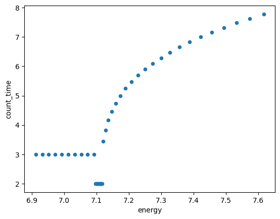
Make a plot of count time v energy using the DEFAULT_XAFS_SCAN_SEGMENTS. See how the count time changes throughout the post-edge region due to use of kwt (k-weighted count time) axis.

e_arr, t_arr = parse_segments(7.1125, DEFAULT_XAFS_SCAN_SEGMENTS)
df = pd.DataFrame(dict(energy=e_arr, count_time=t_arr))
df.plot.scatter("energy", "count_time")

<Axes: xlabel='energy', ylabel='count_time'>

real-time computation of absorption coefficient

The absorption coefficient is computed from the ratio of two scaler channels. We could compute that either in Python or EPICS. Here, we choose an EPICS userCalc because its setup is more familiar to people experienced with EPICS. The instrument package already provides support for 10 userCalcs. We’ll pick userCalc2 (since userCalc1 is already used by the simulated temperature controller).

The computation will update when it gets new values for either scaler channel. In our xafs() scan below, we’ll connect (separately, so we don’t get all the other data provided by the userCalc support) with the calculated value (log(I00/I0)) as an additional detector.

def prep_absorption_calc(absorption):
    """
    Use a userCalc to compute ln(I00/I0) for real-time plots in collection.

    PARAMETERS

    absorption
        obj: instance of apstools.synApps.SwaitRecord()
    """
    absorption.reset()
    s = scaler1.channels
    yield from bps.mv(
        absorption.channels.A.input_pv, s.chan02.s.pvname,  # I0
        absorption.channels.B.input_pv, s.chan06.s.pvname,  # I00
        absorption.calculation, "ln(B/A)",  # ln(I00/I0)
        absorption.scanning_rate, "I/O Intr",
    )

xafs() plan

With all the pieces defined, it is time to write a plan to measure the XAFS. The caller must provide the absorption edge energy (in keV). A list of segments is optional (will default to DEFAULT_XAFS_SCAN_SEGMENTS as defined above) so only the absorption edge energy is required. Once the inputs are checked for correctness, the absorption calculation is setup in an EPICS userCalc (SwaitRecord). Finally, the 1-D step scan is run by calling bp.list_scan() with lists of energy and count time values for each step.

def xafs(edge_keV, segments=None, detectors=None):
    """
    Scan an edge: (keV

    EXAMPLE::

        RE(xafs(7.1125))  # scan iron K edge
    """
    if detectors is None:
        detectors = [scaler1]
    if segments is None:
        segments = DEFAULT_XAFS_SCAN_SEGMENTS
    if len(segments) == 0:
        return  # nothing to do

    # use userCalc2 to calculate absorption
    absorption = calcs.calc2
    yield from prep_absorption_calc(absorption)

    # override: just get the one signal
    absorption = EpicsSignalRO(
        calcs.calc2.calculated_value.pvname,
        name="absorption",
        kind="hinted"
    )
    detectors.append(absorption)

    scaler1.select_channels(("I0", "I00"))

    energy_list, count_time_list = parse_segments(edge_keV, segments)

    comment = (
        f"xafs of {len(segments)} segments (combined) near {edge_keV} keV"
        f": {len(energy_list)} points total"
    )
    logger.info(comment)
    yield from bp.list_scan(
        detectors,
        dcm.energy, energy_list,
        scaler1.preset_time, count_time_list,
        md=dict(
            purpose=comment,
            plan_name="xafs"
        )
    )

If the IOC was just started, the motor positions may not allow the monochromator code to operate. Let’s check it and move the motors only if necessary.

if (
    dcm.wavelength.position == 0
    and dcm.theta.position == 0
    and dcm.y1.get() == 0
    and dcm.z2.get() == 0
):
    from ophyd import EpicsMotor

    print(f"{dcm.name} is not initialized.  Moving motors to start position.")
    # The DCM controls do not allow operation of the underlying motors directly.
    # Let's move them anyway, just from this code.
    ioc = iconfig.get("GP_IOC_PREFIX")
    m_th = EpicsMotor(f"{ioc}m45", name="m_th")
    m_y1 = EpicsMotor(f"{ioc}m46", name="m_y1")
    m_z2 = EpicsMotor(f"{ioc}m47", name="m_z2")
    m_th.wait_for_connection()
    m_y1.wait_for_connection()
    m_z2.wait_for_connection()

    # we can't use Magicks so use RE to move them together
    # These settings are ~3.7 keV, where th & z2 are comparable
    # which means it takes roughly the same time to reach this position.
    RE(bps.mv(m_th, 32.3, m_y1, -20.7, m_z2, 32.7))

print(f"Initial {dcm.energy.position=:.4f} keV")

Initial dcm.energy.position=7.4563 keV

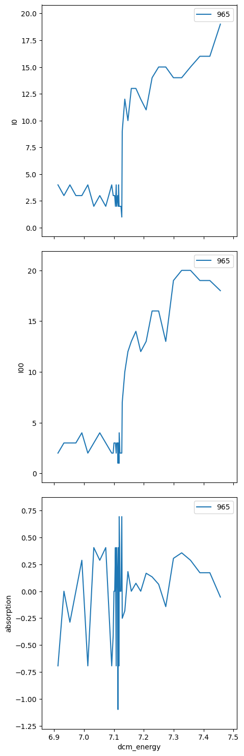
XAFS scan with bluesky

# move near the starting point
RE(bps.mv(dcm.energy, 7))

my_segments = (  # faster than above, just for the demo
    # X could be keV, eV, k, or kwt (k-weighted count time)
    # axis, start, end, step, count_time
    ("keV", -.2, -.015, .02, .6),
    ("eV", -15, 10, 2.5, .5),
    ("k", .5, 2, .2, 0.4),
    ("kwt", 2, 10, .5, .5),
)

# start the scan
RE(xafs(7.1125, segments=my_segments))

I Thu-18:20:05 - xafs of 4 segments (combined) near 7.1125 keV: 44 points total

Transient Scan ID: 965     Time: 2023-04-13 18:20:05
Persistent Unique Scan ID: '13d5ecf4-55dd-41d8-9a96-4231230e6200'
New stream: 'label_start_motor'
New stream: 'primary'
+-----------+------------+------------+------------+------------+------------+
|   seq_num |       time | dcm_energy |         I0 |        I00 | absorption |
+-----------+------------+------------+------------+------------+------------+
|         1 | 18:20:07.9 |     6.9125 |          4 |          2 |   -0.69315 |
|         2 | 18:20:09.6 |     6.9325 |          3 |          3 |    0.00000 |
|         3 | 18:20:11.4 |     6.9525 |          4 |          3 |   -0.28768 |
|         4 | 18:20:13.1 |     6.9725 |          3 |          3 |    0.00000 |
|         5 | 18:20:14.9 |     6.9925 |          3 |          4 |    0.28768 |
|         6 | 18:20:16.7 |     7.0125 |          4 |          2 |   -0.69315 |
|         7 | 18:20:18.4 |     7.0325 |          2 |          3 |    0.40547 |
|         8 | 18:20:20.1 |     7.0525 |          3 |          4 |    0.28768 |
|         9 | 18:20:21.9 |     7.0725 |          2 |          3 |    0.40547 |
|        10 | 18:20:23.7 |     7.0925 |          4 |          2 |   -0.69315 |
|        11 | 18:20:25.2 |     7.0975 |          3 |          2 |   -0.40547 |
|        12 | 18:20:26.6 |     7.1000 |          3 |          3 |    0.00000 |
|        13 | 18:20:28.0 |     7.1025 |          3 |          3 |    0.00000 |
|        14 | 18:20:29.3 |     7.1050 |          2 |          3 |    0.40547 |
|        15 | 18:20:30.7 |     7.1075 |          4 |          2 |   -0.69315 |
|        16 | 18:20:32.1 |     7.1092 |          2 |          3 |    0.40547 |
|        17 | 18:20:33.5 |     7.1125 |          3 |          3 |    0.00000 |
|        18 | 18:20:34.8 |     7.1135 |          3 |          1 |   -1.09861 |
|        19 | 18:20:36.2 |     7.1144 |          2 |          3 |    0.40547 |
|        20 | 18:20:37.5 |     7.1150 |          2 |          3 |    0.40547 |
|        21 | 18:20:38.7 |     7.1156 |          4 |          2 |   -0.69315 |
|        22 | 18:20:40.0 |     7.1171 |          2 |          1 |   -0.69315 |
|        23 | 18:20:41.3 |     7.1175 |          2 |          4 |    0.69315 |
|        24 | 18:20:42.7 |     7.1189 |          2 |          3 |    0.40547 |
|        25 | 18:20:44.2 |     7.1200 |          2 |          2 |    0.00000 |
|        26 | 18:20:45.6 |     7.1211 |          2 |          2 |    0.00000 |
|        27 | 18:20:47.0 |     7.1235 |          2 |          2 |    0.00000 |
|        28 | 18:20:48.4 |     7.1263 |          1 |          2 |    0.69315 |
|        29 | 18:20:51.3 |     7.1277 |          9 |          7 |   -0.25131 |
|        30 | 18:20:54.5 |     7.1363 |         12 |         10 |   -0.18232 |
|        31 | 18:20:57.9 |     7.1468 |         10 |         12 |    0.18232 |
|        32 | 18:21:01.4 |     7.1582 |         13 |         13 |    0.00000 |
|        33 | 18:21:05.1 |     7.1734 |         13 |         14 |    0.07411 |
|        34 | 18:21:09.0 |     7.1896 |         12 |         12 |    0.00000 |
|        35 | 18:21:13.0 |     7.2078 |         11 |         13 |    0.16705 |
|        36 | 18:21:17.1 |     7.2278 |         14 |         16 |    0.13353 |
|        37 | 18:21:21.4 |     7.2497 |         15 |         16 |    0.06454 |
|        38 | 18:21:25.8 |     7.2735 |         15 |         13 |   -0.14310 |
|        39 | 18:21:30.2 |     7.2992 |         14 |         19 |    0.30538 |
|        40 | 18:21:34.9 |     7.3268 |         14 |         20 |    0.35667 |
|        41 | 18:21:39.7 |     7.3563 |         15 |         20 |    0.28768 |
|        42 | 18:21:44.6 |     7.3878 |         16 |         19 |    0.17185 |
|        43 | 18:21:49.5 |     7.4211 |         16 |         19 |    0.17185 |
|        44 | 18:21:54.5 |     7.4563 |         19 |         18 |   -0.05407 |
+-----------+------------+------------+------------+------------+------------+
generator xafs ['13d5ecf4'] (scan num: 965)

('13d5ecf4-55dd-41d8-9a96-4231230e6200',)

Challenges

1. Scan XAFS with 3 segments (below-edge, near-edge, above-edge regions).

2. Explain why we can’t we scan in negative k-space.

3. Modify the software to allow the user to control the k weighting terms: factor and exponent.

4. Modify the xafs() plan to accept user metadata. (hint: provide for a md keyword argument that will be a dictionary. See bp.list_scan?? for an example.)

References

• https://docs.xrayabsorption.org/tutorials/XAFS_Fundamentals.pdf

• https://docs.xrayabsorption.org/Workshops/IIT2013/Newville_Theory.pdf

• https://en.wikipedia.org/wiki/X-ray_absorption_fine_structure

• web tool: https://nbeaver.github.io/k-space-calculator/

• nbeaver/k-space-calculator