Fly Scans with EPICS motor and scaler#

The ScalerMotorFlyer() device from apstools makes it possible to run fly scans with just the EPICS motor and scaler records.

This combination of positioner and detector represent common EPICS support available to most APS beam lines. An external fly scan controller is not necessary, nor is any dedicated data collection hardware. Keep in mind that the capabilities of the motor and scaler will provide certain limits on how fast the scan completes and how many data points may be collected.

Contents

What is a bluesky/ophyd ‘Flyer’?
Step-by-step outline of ‘ScalerMotorFlyer()’
Prepare the session
Run the fly scan
Get the data and plot it

Overview#

Q: What is a bluesky/ophyd ``Flyer``?

A bluesky/ophyd Flyer is an ophyd Device which describes a data collection process that is not managed by the bluesky RunEngine. Examples of such data collection processes include:

A system using dedicated hardware to control the measurement sequence and collect data.
Some software that can be called from Python.
A Python function that runs in a background thread.

The Flyer interfaces with the RunEngine with these three distinct steps:

kickoff() : Start the fly scan.
complete() : Wait for the fly scan to complete.
collect() : Get (and report) the fly scan data.

Note: There is an additional step, describe_collect(), which informs bluesky about the type(s) of data reported by collect().

In ScalerMotorFlyer(), the fly scan protocol is managed by the actions_thread() method. This method is run in its own thread so it does not interfere with the bluesky RunEngine.

Outline#

Here is a step-by-step outline of the fly scan protocol:

Setup
1. Scaler update rate is set from the requested sampling period.
Taxi
1. Motor is sent to the start position (using original velocity).
2. Wait for motor to reach start position.
Fly
1. Motor velocity is set based on the requested start & finish positions and fly_time for the scan.
2. Scaler count time set to fly_time plus a smidgen (scaler_time_pad).
3. Start periodic data collection
  1. Scaler provides (EPICS Channel Access) updates as new data is available.
  2. Record motor position & scaler channel counts.
  3. Record time stamps for motor and scaler (probably different).
  4. Data accumulated to internal memory.
4. Scaler is started to count.
5. Motor is sent to finish (using fly scan velocity).
6. Wait for motor to stop moving.
7. Scaler is stopped.
8. Stop periodic data collection
Finish
1. Reset to previous values
  1. motor velocity
  2. scaler update rate
2. Report any acquired data to Bluesky RunEngine.
  1. Data for each counter is reported as the difference of successive readings.

If any exceptions are raised by steps 1-3 (such as cannot set a value, timeout, wrong type of parameter given, …), skip directly to step 4.

Setup#

Without more explanation here, we set up our bluesky session for data acquisition, importing needed libraries and constructing the RunEngine and databroker for a temporary catalog. We will use an EPICS IOC with the prefix gp:. This IOC provides a simulated motor and a simulated scaler, among other features. The scaler is preconfigured with detector inputs. When the scaler is counting, its counters (detector channels) are updated by random integers.

[1]:

%matplotlib inline
from apstools.devices import make_dict_device
from apstools.devices import ScalerMotorFlyer
from bluesky import plan_stubs as bps
from bluesky import plans as bp
from bluesky import preprocessors as bpp
from bluesky import RunEngine
from bluesky.callbacks.best_effort import BestEffortCallback
from matplotlib import pyplot as plt
from ophyd import EpicsMotor
from ophyd.scaler import ScalerCH
import databroker

IOC = "gp:"

# ophyd-level
m1 = EpicsMotor(f"{IOC}m10", name="motor")
scaler = ScalerCH(f"{IOC}scaler1", name="scaler")
m1.wait_for_connection()
scaler.wait_for_connection()
scaler.select_channels()

# bluesky-level
cat = databroker.temp().v2
plt.ion()  # enables matplotlib graphics
RE = RunEngine({})
RE.subscribe(cat.v1.insert)
best_effort_callback = BestEffortCallback()
RE.subscribe(best_effort_callback)  # LivePlot & LiveTable

[1]:

Create the flyer object that will be used by the bluesky fly() plan. The ScalerMotorFlyer() deivce supports the ophyd flyer interface, as described above.

In this example, we describe a fly scan from motor position 1 to 5 that should take 4 seconds, collecting data at 0.1 second intervals. Other keyword parameters are accepted. See the documentation for full details.

[2]:

flyer = ScalerMotorFlyer(scaler, m1, 1, 5, fly_time=4, period=.1, name="flyer")

Augment the standard (a.k.a. bluesky pre-assembled) `bp.fly() <https://blueskyproject.io/bluesky/generated/bluesky.plans.fly.html#bluesky.plans.fly>`__ plan to save the peak statistics to a separate stream in the run after the fly scan is complete.

[3]:

def fly_with_stats(flyers, *, md=None):
    """Replaces bp.fly(), adding stream for channel stats."""

    @bpp.stage_decorator(flyers)
    @bpp.run_decorator(md=md)
    @bpp.stub_decorator()
    def _inner_fly():
        yield from bp.fly(flyers)
        for flyer in flyers:
            if hasattr(flyer, "stats") and isinstance(flyer.stats, dict):
                yield from _flyer_stats_stream(flyer, f"{flyer.name}_stats")

    def _flyer_stats_stream(flyer, stream=None):
        """Output stats from this flyer into separate stream."""
        yield from bps.create(name=stream or f"{flyer.name}_stats")
        for ch in list(flyer.stats.keys()):
            yield from bps.read(
                make_dict_device(
                    {
                        # fmt: off
                        stat: v
                        for stat, v in flyer.stats[ch].to_dict().items()
                        if v is not None
                        # fmt: on
                    },
                    name=ch
                )
            )
        yield from bps.save()

    yield from _inner_fly()

Scan#

Using our flyer device with the bluesky fly() plan, run the fly scan. Supply additional metadata so we can label our plot. The call to RE() returns a list of the uids for each run that was executed. Collect this list (we expect only one uid in the list) for later use when accessing the run from the databroker.

[4]:

uids = RE(fly_with_stats([flyer], md=dict(title="Demonstrate a scaler v. motor fly scan.")))



Transient Scan ID: 1     Time: 2022-12-14 12:42:21
Persistent Unique Scan ID: '50b5225e-f698-46c2-9b54-c2038e635826'
New stream: 'primary'
+-----------+------------+
|   seq_num |       time |
+-----------+------------+

/home/prjemian/micromamba/envs/bluesky_2022_3/lib/python3.9/site-packages/event_model/__init__.py:208: UserWarning: The document type 'bulk_events' has been deprecated in favor of 'event_page', whose structure is a transpose of 'bulk_events'.
  warnings.warn(

New stream: 'flyer_stats'
+-----------+------------+
generator fly_with_stats ['50b5225e'] (scan num: 1)

Note that the LiveTable and LivePlot from the BestEffortCallback do not yet know how to show this data, so they report minimal information about the fly scan.

Visualize#

To make a plot of the data, first get the run from the databroker, identified here by its uid.

[5]:

run = cat.v2[uids[0]]
run

[5]:

BlueskyRun
  uid='50b5225e-f698-46c2-9b54-c2038e635826'
  exit_status='success'
  2022-12-14 12:42:21.253 -- 2022-12-14 12:42:29.889
  Streams:
    * flyer_stats
    * primary

Show some of the run’s metadata, verifying that we are looking at the run we just acquired.

[6]:

print(f"{run.metadata['start']['scan_id']=}")
print(f"{run.metadata['start']['title']=}")

run.metadata['start']['scan_id']=1
run.metadata['start']['title']='Demonstrate a scaler v. motor fly scan.'

The run has a single stream of data, named primary. Get the data from that stream:

[7]:

dataset = run.primary.read()
dataset

Choose data for the x and y axes from the dataset names:

[8]:

x = dataset["motor"]
y = dataset["diode"]

Plot the data using matplotlib’s pyplot module. (The pyplot as plt library was imported above.)

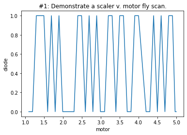
[9]:

title = (
    f"#{run.metadata['start']['scan_id']}"
    f": {run.metadata['start']['title']}"
)
plt.plot(x.values, y.values)
plt.title(title)
plt.xlabel(x.name)
plt.ylabel(y.name)

[9]:

Text(0, 0.5, 'diode')

../_images/examples_de_scaler_motor_flyer_21_1.png

Show statistics collected for each scaler channel.

[10]:

run.flyer_stats.read()

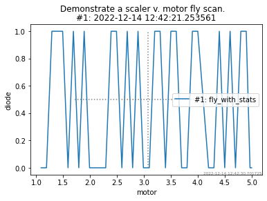
There’s a new utility function apstools since version 1.6.10: plotxy() does all these steps. Returns the exact, same results for just the named signals, plus a computed fwhm = 2*sigma*sqrt(2ln(2)). Lines are drawn at the centroid and fwhm.

[11]:

from apstools.utils import plotxy
plotxy(run, "motor", "diode")

[11]:

{1: {'mean_x': 3.0456097560975612,
  'mean_y': 0.4634146341463415,
  'stddev_x': 1.2126995686906301,
  'stddev_y': 0.5048544827774513,
  'slope': 0.009237722080560458,
  'intercept': 0.4352801376536687,
  'correlation': 0.02218972390053605,
  'centroid': 3.0742105263157895,
  'sigma': 1.1539466182557723,
  'min_x': 1.09,
  'max_x': 5.0,
  'min_y': 0.0,
  'max_y': 1.0,
  'x_at_max_y': 4.9,
  'fwhm': 2.7173366275643693}}

../_images/examples_de_scaler_motor_flyer_25_1.png