The lineup2() plan — align an axis with a signal

The apstools.plans.lineup2() plan aligns a mover (axis) to the peak of a detector signal. It scans mover over a relative range, computes peak statistics using numpy, and moves the mover to the chosen statistical feature (default: "centroid"). If nscans > 1 (default: 2), a second, finer scan is run centred on the result of the first.

Unlike the older, deprecated lineup() plan, lineup2():

• does not require a BestEffortCallback,

• works in the queueserver, Jupyter notebooks, and IPython consoles,

• writes peak statistics as a named bluesky stream ("signal_stats" by default) before the run closes, so they are available in the data catalog immediately after each scan.

This notebook uses only simulated (software-only) devices — no EPICS hardware is required.

Setup

%matplotlib inline
import warnings

warnings.filterwarnings("ignore", category=FutureWarning)
import databroker
from bluesky import RunEngine
from bluesky.callbacks import best_effort
from ophyd.sim import SynGauss
from ophyd import SoftPositioner

from apstools.plans import lineup2

cat = databroker.temp()
RE = RunEngine({})
RE.subscribe(cat.v1.insert)

bec = best_effort.BestEffortCallback()
RE.subscribe(bec)

1

Create a simulated mover and a Gaussian detector signal centred at x = -0.5.

m1 = SoftPositioner(name="m1", init_pos=0.0)

noisy = SynGauss(
    "noisy",
    m1,
    "m1",
    center=-0.5,
    Imax=1e5,
    sigma=0.1,
    noise="poisson",
)
noisy.kind = "hinted"

Run lineup2()

Scan m1 over ±2 around its current position with 41 points and two passes. Peak statistics are printed after each pass and are also written as the "signal_stats" bluesky stream before the run closes.

RE(lineup2([noisy], m1, -2, 2, 41))

Transient Scan ID: 1     Time: 2026-03-27 11:08:23
Persistent Unique Scan ID: '36cb71fa-7b53-4df6-8cc6-a50941f7c8a5'
New stream: 'primary'
+-----------+------------+------------+
|   seq_num |       time |      noisy |
+-----------+------------+------------+
|         1 | 11:08:23.2 |          0 |
|         2 | 11:08:23.3 |          0 |
|         3 | 11:08:23.3 |          0 |
|         4 | 11:08:23.3 |          0 |

|         5 | 11:08:23.4 |          0 |
|         6 | 11:08:23.4 |          0 |
|         7 | 11:08:23.5 |          0 |
|         8 | 11:08:23.5 |          0 |
|         9 | 11:08:23.6 |          0 |

|        10 | 11:08:23.6 |          0 |
|        11 | 11:08:23.6 |          0 |
|        12 | 11:08:23.7 |         33 |
|        13 | 11:08:23.7 |       1154 |
|        14 | 11:08:23.8 |      13617 |

|        15 | 11:08:23.8 |      60446 |
|        16 | 11:08:23.9 |      99782 |
|        17 | 11:08:23.9 |      60687 |
|        18 | 11:08:24.0 |      13381 |
|        19 | 11:08:24.0 |       1103 |

|        20 | 11:08:24.0 |         35 |
|        21 | 11:08:24.1 |          0 |
|        22 | 11:08:24.1 |          0 |
|        23 | 11:08:24.2 |          0 |
|        24 | 11:08:24.2 |          0 |
|        25 | 11:08:24.2 |          0 |

|        26 | 11:08:24.3 |          0 |
|        27 | 11:08:24.3 |          0 |
|        28 | 11:08:24.4 |          0 |
|        29 | 11:08:24.4 |          0 |
|        30 | 11:08:24.5 |          0 |

|        31 | 11:08:24.5 |          0 |
|        32 | 11:08:24.5 |          0 |
|        33 | 11:08:24.6 |          0 |
|        34 | 11:08:24.6 |          0 |
|        35 | 11:08:24.7 |          0 |

|        36 | 11:08:24.7 |          0 |
|        37 | 11:08:24.8 |          0 |
|        38 | 11:08:24.8 |          0 |
|        39 | 11:08:24.8 |          0 |
|        40 | 11:08:24.9 |          0 |

|        41 | 11:08:24.9 |          0 |
New stream: 'signal_stats'
+-----------+------------+------------+
Plan lineup2 ['36cb71fa'] (scan num: 1)

Motor: 'm1'  Detector: 'noisy'  Feature: 'centroid'
========== ======================
statistic  value                 
========== ======================
n          41                    
centroid   -0.5001502569553784   
x_at_max_y -0.5                  
fwhm       0.2453610814405645    
variance   0.010011486466238052  
sigma      0.10005741584829209   
min_x      -2.0                  
mean_x     1.0831444142684454e-16
max_x      2.0                   
min_y      0                     
mean_y     6103.365853658536     
max_y      99782                 
========== ======================

m1 moved to centroid: -0.5001502569553784


Transient Scan ID: 2     Time: 2026-03-27 11:08:25
Persistent Unique Scan ID: '4cd1e16c-301e-431f-88b6-c8bca8fda6b6'
New stream: 'primary'
+-----------+------------+------------+
|   seq_num |       time |      noisy |
+-----------+------------+------------+
|         1 | 11:08:25.2 |          0 |
|         2 | 11:08:25.2 |          4 |
|         3 | 11:08:25.3 |          8 |
|         4 | 11:08:25.3 |         21 |

|         5 | 11:08:25.4 |         41 |
|         6 | 11:08:25.4 |        106 |
|         7 | 11:08:25.5 |        266 |
|         8 | 11:08:25.5 |        612 |
|         9 | 11:08:25.6 |       1280 |

|        10 | 11:08:25.6 |       2671 |
|        11 | 11:08:25.7 |       4996 |
|        12 | 11:08:25.7 |       8837 |
|        13 | 11:08:25.8 |      14331 |
|        14 | 11:08:25.8 |      22751 |

|        15 | 11:08:25.9 |      34167 |
|        16 | 11:08:25.9 |      47339 |
|        17 | 11:08:25.9 |      61833 |
|        18 | 11:08:26.0 |      76316 |
|        19 | 11:08:26.0 |      88850 |

|        20 | 11:08:26.1 |      96750 |
|        21 | 11:08:26.1 |     100382 |
|        22 | 11:08:26.2 |      96945 |
|        23 | 11:08:26.2 |      89043 |
|        24 | 11:08:26.3 |      76557 |

|        25 | 11:08:26.3 |      61925 |
|        26 | 11:08:26.4 |      47149 |
|        27 | 11:08:26.4 |      33712 |
|        28 | 11:08:26.5 |      22614 |
|        29 | 11:08:26.5 |      14654 |

|        30 | 11:08:26.6 |       8755 |
|        31 | 11:08:26.6 |       4780 |
|        32 | 11:08:26.7 |       2691 |
|        33 | 11:08:26.7 |       1256 |
|        34 | 11:08:26.8 |        584 |

|        35 | 11:08:26.8 |        286 |
|        36 | 11:08:26.8 |        116 |
|        37 | 11:08:26.9 |         44 |
|        38 | 11:08:26.9 |         34 |
|        39 | 11:08:27.0 |          9 |

|        40 | 11:08:27.0 |          1 |
|        41 | 11:08:27.1 |          2 |
New stream: 'signal_stats'
+-----------+------------+------------+
Plan lineup2 ['4cd1e16c'] (scan num: 2)

Motor: 'm1'  Detector: 'noisy'  Feature: 'centroid'
========== =====================
statistic  value                
========== =====================
n          41                   
centroid   -0.5002225420758496  
x_at_max_y -0.5001502569553784  
fwhm       0.23548172867948947  
variance   0.009987929441983073 
sigma      0.09993962898661908  
min_x      -0.9908724198365074  
mean_x     -0.5001502569553784  
max_x      -0.009428094074249382
min_y      0                    
mean_y     24944.341463414636   
max_y      100382               
========== =====================

m1 moved to centroid: -0.5002225420758496

('36cb71fa-7b53-4df6-8cc6-a50941f7c8a5',
 '4cd1e16c-301e-431f-88b6-c8bca8fda6b6')

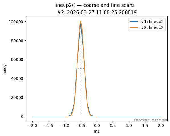
Plot

Use apstools.utils.plotxy() to overlay both scans. The coarse first scan (wide range) and the fine second scan (narrow range, centred on the result of the first) are plotted together. Centroid and FWHM markers are added automatically when stats=True (the default).

from apstools.utils import plotxy

# Plot the coarse scan first, then overlay the fine scan.
plotxy(cat.v2[-2], "m1", "noisy", title="lineup2() — coarse and fine scans")
plotxy(cat.v2[-1], "m1", "noisy", append=True);

Inspect the signal_stats stream

Because lineup2() writes peak statistics into the "signal_stats" stream before each run closes, they are immediately available from the catalog. The most recent run’s statistics can be read like any other bluesky stream:

run = cat.v2[-1]
run.signal_stats.read()

<xarray.Dataset> Size: 201B
Dimensions:                                (time: 1)
Coordinates:
  * time                                   (time) float64 8B 1.775e+09
Data variables: (12/25)
    lineup2_signal_stats_max_x             (time) float64 8B -0.009428
    lineup2_signal_stats_mean_x            (time) float64 8B -0.5002
    lineup2_signal_stats_median_x          (time) float64 8B -0.5002
    lineup2_signal_stats_min_x             (time) float64 8B -0.9909
    lineup2_signal_stats_n                 (time) int64 8B 41
    lineup2_signal_stats_range_x           (time) float64 8B 0.9814
    ...                                     ...
    lineup2_signal_stats_correlation       (time) float64 8B -0.0001836
    lineup2_signal_stats_intercept         (time) float64 8B 2.493e+04
    lineup2_signal_stats_slope             (time) float64 8B -21.39
    lineup2_signal_stats_stddev_intercept  (time) float64 8B 1.079e+04
    lineup2_signal_stats_stddev_slope      (time) float64 8B 1.866e+04
    lineup2_signal_stats_success           (time) bool 1B True

xarray.Dataset

• Dimensions:
  • time: 1
• Coordinates: (1)
  • time
    (time)
    float64
    1.775e+09

    array([1.774628e+09])

• Data variables: (25)
  • lineup2_signal_stats_max_x
    (time)
    float64
    -0.009428

    object :

    lineup2_signal_stats

    array([-0.00942809])

  • lineup2_signal_stats_mean_x
    (time)
    float64
    -0.5002

    object :

    lineup2_signal_stats

    array([-0.50015026])

  • lineup2_signal_stats_median_x
    (time)
    float64
    -0.5002

    object :

    lineup2_signal_stats

    array([-0.50015026])

  • lineup2_signal_stats_min_x
    (time)
    float64
    -0.9909

    object :

    lineup2_signal_stats

    array([-0.99087242])

  • lineup2_signal_stats_n
    (time)
    int64
    41

    object :

    lineup2_signal_stats

    array([41])

  • lineup2_signal_stats_range_x
    (time)
    float64
    0.9814

    object :

    lineup2_signal_stats

    array([0.98144433])

  • lineup2_signal_stats_stddev_x
    (time)
    float64
    0.2903

    object :

    lineup2_signal_stats

    array([0.29031515])

  • lineup2_signal_stats_max_y
    (time)
    int64
    100382

    object :

    lineup2_signal_stats

    array([100382])

  • lineup2_signal_stats_mean_y
    (time)
    float64
    2.494e+04

    object :

    lineup2_signal_stats

    array([24944.34146341])

  • lineup2_signal_stats_median_y
    (time)
    float64
    5.019e+04

    object :

    lineup2_signal_stats

    array([50191.])

  • lineup2_signal_stats_min_y
    (time)
    int64
    0

    object :

    lineup2_signal_stats

    array([0])

  • lineup2_signal_stats_range_y
    (time)
    int64
    100382

    object :

    lineup2_signal_stats

    array([100382])

  • lineup2_signal_stats_stddev_y
    (time)
    float64
    3.383e+04

    object :

    lineup2_signal_stats

    array([33831.92875161])

  • lineup2_signal_stats_x_at_min_y
    (time)
    float64
    -0.9909

    object :

    lineup2_signal_stats

    array([-0.99087242])

  • lineup2_signal_stats_x_at_max_y
    (time)
    float64
    -0.5002

    object :

    lineup2_signal_stats

    array([-0.50015026])

  • lineup2_signal_stats_centroid
    (time)
    float64
    -0.5002

    object :

    lineup2_signal_stats

    array([-0.50022254])

  • lineup2_signal_stats_fwhm
    (time)
    float64
    0.2355

    object :

    lineup2_signal_stats

    array([0.23548173])

  • lineup2_signal_stats_variance
    (time)
    float64
    0.009988

    object :

    lineup2_signal_stats

    array([0.00998793])

  • lineup2_signal_stats_sigma
    (time)
    float64
    0.09994

    object :

    lineup2_signal_stats

    array([0.09993963])

  • lineup2_signal_stats_correlation
    (time)
    float64
    -0.0001836

    object :

    lineup2_signal_stats

    array([-0.00018358])

  • lineup2_signal_stats_intercept
    (time)
    float64
    2.493e+04

    object :

    lineup2_signal_stats

    array([24933.64150577])

  • lineup2_signal_stats_slope
    (time)
    float64
    -21.39

    object :

    lineup2_signal_stats

    array([-21.39348624])

  • lineup2_signal_stats_stddev_intercept
    (time)
    float64
    1.079e+04

    object :

    lineup2_signal_stats

    array([10791.44049877])

  • lineup2_signal_stats_stddev_slope
    (time)
    float64
    1.866e+04

    object :

    lineup2_signal_stats

    array([18660.56339487])

  • lineup2_signal_stats_success
    (time)
    bool
    True

    object :

    lineup2_signal_stats

    array([ True])

Validate

Confirm that m1 was moved to within one sigma of the known peak centre.

center = -0.5  # known centre of the simulated Gaussian
sigma = 0.1  # known sigma

print(f"Peak centre: {center}   m1 position: {m1.position:.4f}")
print(f"Alignment successful: {abs(m1.position - center) < sigma}")
assert abs(m1.position - center) < sigma

Peak centre: -0.5   m1 position: -0.5002
Alignment successful: True