User Guide#
Getting Started#
mdaviz is a Python Qt6 application for visualizing MDA (Multi-Dimensional Array) data.
Installation#
For installation instructions, see the Installation Guide page.
Running the Application#
After installation, you can run mdaviz in several ways:
From PyPI installation:
conda activate mdaviz
mdaviz
From source installation:
conda activate mdaviz
cd mdaviz
mdaviz
At the Advanced Photon Source:
/APSshare/bin/mdaviz
Basic Usage#
Opening Data#
Auto-Load: The application automatically loads the first valid folder from your recent folders list. This can be enabled/disabled in the preferences.
Manual Open: Use the recent folder dropdown to select a file in a different folder or click “Open…” or the icon to browse.
Recent Folders: The dropdown shows your recently opened folders for quick access.
Data Visualization#
Plot Mode: Choose between Auto-replace, Auto-add, or Auto-off (i.e. add/replace manually) modes.
Add to graph: In Auto-replace mode, hold CTRL (CMD on macOS) while clicking a file to overlay its curves on the current plot. In Auto-add mode, clicking a file always adds its curves to the plot.
Live plotting: When a scan is acquiring, the plot updates automatically every 2 seconds as new data points are recorded. A red ● LIVE HH:MM:SS indicator appears in the chart title during live updates. You can overlay curves from other scans using CTRL+click without interrupting the live update.
Data Selection: Use the checkbox columns to control what’s plotted:
X: Positioner (only one allowed)
Y: Detector (multiple allowed)
I0: Select for normalization (divide Y data by this field, only one allowed)
Un: Unscale curves to match the range of other Y curves (requires Y selection on same row)
Interactive Plot: Use matplotlib’s interactive features for zooming, panning, and changing figure options.
Data Processing Options:
I0 Normalization: Divide Y data by the selected I0 field to normalize intensity.
Curve Unscaling: Rescale selected curves to match the range of other Y curves.
Select the curve to unscale from the curve dropdown
Check the unscale checkbox in the Basic tab
The unscaling formula:
g(x) = ((f(x) - m) / (M - m)) * (Mg - mg) + mgm, M: min/max of the curve being unscaled f(x)
mg, Mg: global min/max of other Y curves (excluding unscaled ones)
Derivative:
Select a curve from the curve dropdown
Check the derivative checkbox in the Basic tab
Factor/Offset: Open the Basic tab and apply a factor and/or offset to the selected curve (from the curve dropdown)
g(x) = f(x) * factor + offset
Curve Management#
The following options apply to the selected curve in the curve dropdown (top left).
Remove Curve#
Select Curve: Choose the curve to remove from the curve dropdown.
Remove Curve: Click the button.
Curve Style#
Select Curve: Choose a curve from the curve dropdown.
Curve Style: Choose between lines, markers, or both in the “Style” dropdown.
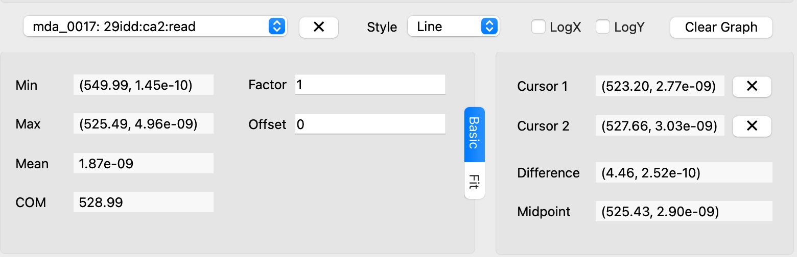
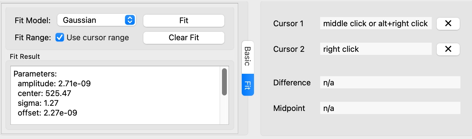
Cursor Utilities#
Cursors snap to the nearest data point of the selected curve
Select Curve: Choose a curve from the curve dropdown.
Cursor 1: Middle-click or alt+right-click to set the first cursor position
Cursor 2: Right-click to set the second cursor position
Range Selection: Use cursors to define fitting ranges
Data Analysis: View mathematical information between cursor positions (difference between cursors & midpoint)
Remove Cursor: Click the button next to the cursor value.
Basic Statistics#
Select Curve: Choose a curve from the curve dropdown.
Basic Statistics: View basic statistics of the curve in the “Basic” tab: min, max, mean, COM.
Factor / Offset#
Select Curve: Choose a curve to transform from the curve dropdown.
Data scaling: Open the Basic tab and apply a factor and/or offset to the selected curve:
f(x) = f(x) * factor + offset.
Curve Fitting#
Select Curve: Choose the curve to fit from the curve dropdown.
Choose Model: Select a fit model from the “Fit Model” dropdown in the “Fit” tab.
Set Range (optional): Check “Use cursor range” if you want to fit only a portion of the data.
Perform Fit: Click the “Fit” button.
View Results: The fit results will appear in the “Fit Results” section
Available models: Gaussian, Lorentzian, Linear, Exponential, Quadratic, Cubic, Error Function.
2D Data Visualization#
Load 2D Data: Open an MDA file containing multi-dimensional data.
Choose Visualization Mode:
1D Slices: Select the 1D tab for line plots
2D Maps: Select the 2D tab for 2D maps
For 1D Slices:
Select the (inner) positioner and detector(s) to plot
Use the spinbox to select the outer positioner value
For 2D Maps:
Use the dropdowns to select the positioner and detector to plot
Choose between heatmap or contour plot display
Adjust color scale or select log scale as needed
Optionally, apply normalization by selecting a detector as I0
For 2D mapping, the data should have more than 1 point in the outer dimension
Troubleshooting#
Common Issues#
Application won’t start:
Ensure PyQt6 is properly installed: pip install PyQt6 Qt6
Check conda environment is activated: conda activate mdaviz
Verify Python version (3.10+ required)
No data displayed:
Check that the selected folder contains MDA files
Check that the selected file is not corrupted (no points in the file) or contains only one point
Verify file permissions
Try refreshing the folder view
After switching from the 2D tab to the 1D tab, basic statistics (min, max, mean, COM) may display “n/a” for curves that were previously working correctly.
Workaround: manipulate the curve in any way (change style, offset, factor, or apply a fit)
The plotting area sometimes expands vertically beyond reasonable bounds:
Workaround: set the maximum plot height to a reasonable value (e.g., 600 pixels) in the preferences
Fitting fails:
Ensure sufficient data points (at least 3 per parameter)
Try a different fit model
Check for invalid data values
Performance issues:
Large datasets may take time to load
Testing & Development#
To run all tests:
pytest src/tests
To run code quality checks:
pre-commit run --all-files
To run type checking:
mypy src/mdaviz
Contributing#
Fork the repository and create a branch for your feature or bugfix.
Add or update tests for your changes.
Run pre-commit, mypy and pytest to ensure all checks pass.
Submit a pull request on GitHub.
For detailed contributing guidelines, see the project’s GitHub repository.
Logging and Debugging#
Default Behavior: By default, mdaviz logs at the WARNING level, showing only warnings, errors and critical messages (quiet mode).
Command Line Options:
You can control the logging level using the --log argument:
# Show only errors and critical messages
mdaviz --log error

# Show warnings, errors, critical messages and info (progress messages, file loading status, and important application events).
mdaviz --log info

# Show all messages including debug information
mdaviz --log debug
Available Log Levels:
debug: Most verbose - shows all messages including detailed debugging information
info: Shows warnings, errors, critical messages, progress, file operations, and general application status
warning: Default level - shows warnings, errors, and critical messages
error: Shows only errors and critical messages
critical: Shows only critical errors
Environment Variables: You can also enable debug mode using the environment variable:
# Enable debug mode via environment variable
export MDAVIZ_DEBUG=1
mdaviz
Log Files:
Log files are automatically created in ~/.mdaviz/logs/ with timestamps. Old log files (older than 1 day) are automatically cleaned up on startup.